mlr3 vis development
Linlin Yin
2019-07-04
mlr3vis_dev.Rmd#devtools::load_all("d:/source/mlr3vis/")
library(mlr3)
library(mlr3vis)
#> Loading required package: data.table
#> Loading required package: ggplot2
#> Loading required package: ggpubr
#> Loading required package: magrittr
#> Registered S3 method overwritten by 'GGally':
#> method from
#> +.gg ggplot2
#> mlr3vis global settings: mlr_plot_theme=theme_pubrmlr: https://mlr.mlr-org.com/articles/tutorial/predict.html
mlr3: https://mlr3book.mlr-org.com/
Learner and Task related
plotLearnerPrediction
This function need learner and task as input. The goal of this function is to show the priediction results with distribution of interested features. It is similar as the function with same name in mlr but it used orginal model in learner (usually used all features) rather than make a new model based on only two interested features. The interestedFeatures were only used for visulization purpose as X axis and Y axis. To show the distribution of prediction result or probability with changes of interested features, grid with different colours were plotted as background. The prediction of grid used orginal model in learner, and interestedFeatures among X and Y axis as data. The median values or most common values for Features used in model but not in interestedFeatures were used to paticipate prediction of the grid background.
Parameters:
* learner: need to be trained and predict_type = “prob”
* task: task, no requirement
* prob.alpha: FALSE shows prediction result; TRUE shows maximal probability
task = mlr_tasks$get("iris")
learner = mlr_learners$get("classif.rpart")
learner$predict_type = "prob"
learner$train(task)
#> <LearnerClassifRpart:classif.rpart>
#> Model: rpart
#> Parameters: xval=0
#> Packages: rpart
#> Predict Type: prob
#> Feature types: logical, integer, numeric, character, factor,
#>   ordered
#> Properties: importance, missings, multiclass, selected_features,
#>   twoclass, weights

plotLearnerPrediction(learner=learner,task=task,prob.alpha = FALSE)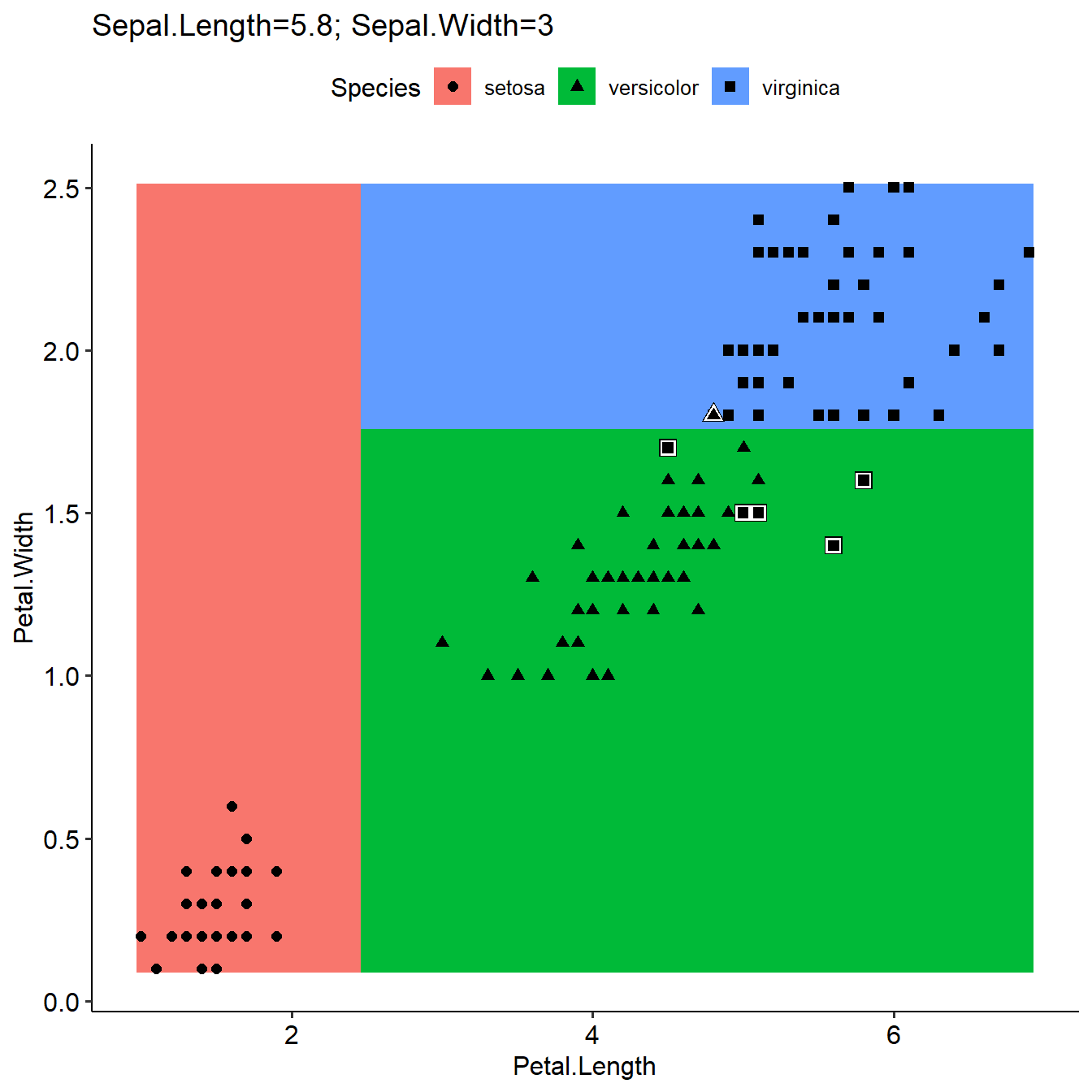
Define otherFeaturesValue for grid prediction in plotLearnerPrediction
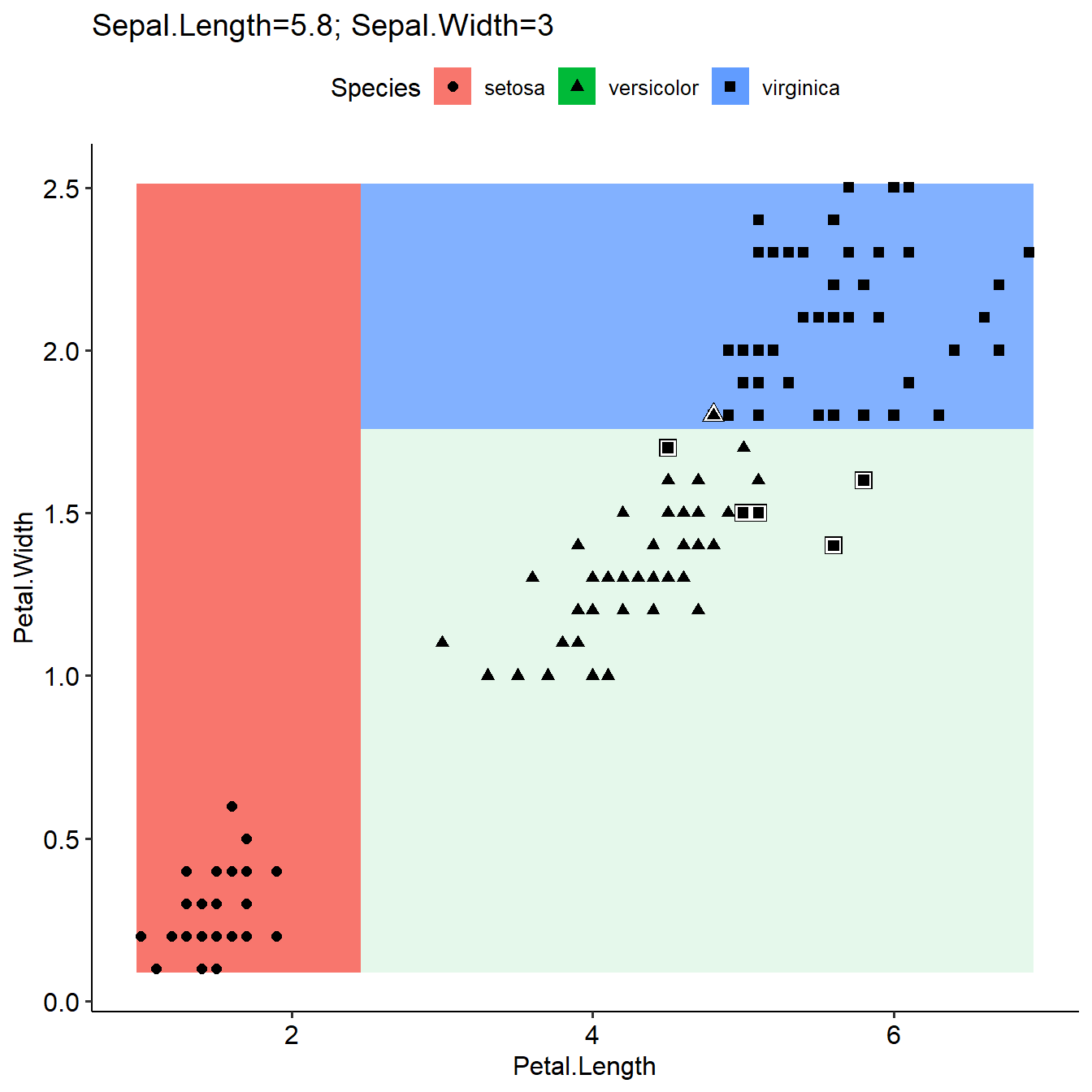
As introduced in last section, plotLearnerPrediction used median or most common value for grid prediction if more than the two interested features were used in the model. Here we can define the values as other Features in the model by a list, and the grid prediction will be based on these values. The results will be different (first figure, not defined otherFeaturesValue, use median value; second figure, use defined otherFeaturesValue).
plotLearnerPrediction(learner=learner,task=task,prob.alpha = TRUE,interestedFeatures= c("Petal.Width","Sepal.Length"))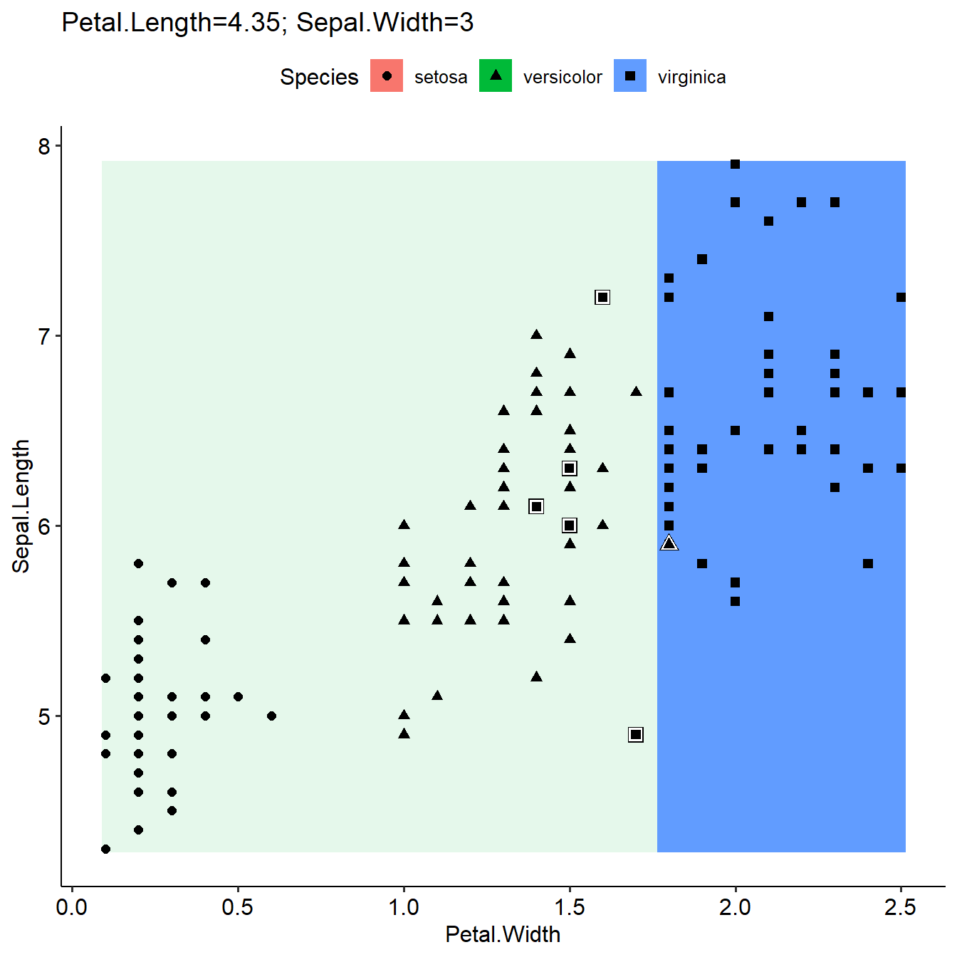
otherFeaturesValue=list(Petal.Length=2.1,Sepal.Width=3.3)
plotLearnerPrediction(learner=learner,task=task,prob.alpha = TRUE,interestedFeatures= c("Petal.Width","Sepal.Length"),otherFeaturesValue=otherFeaturesValue)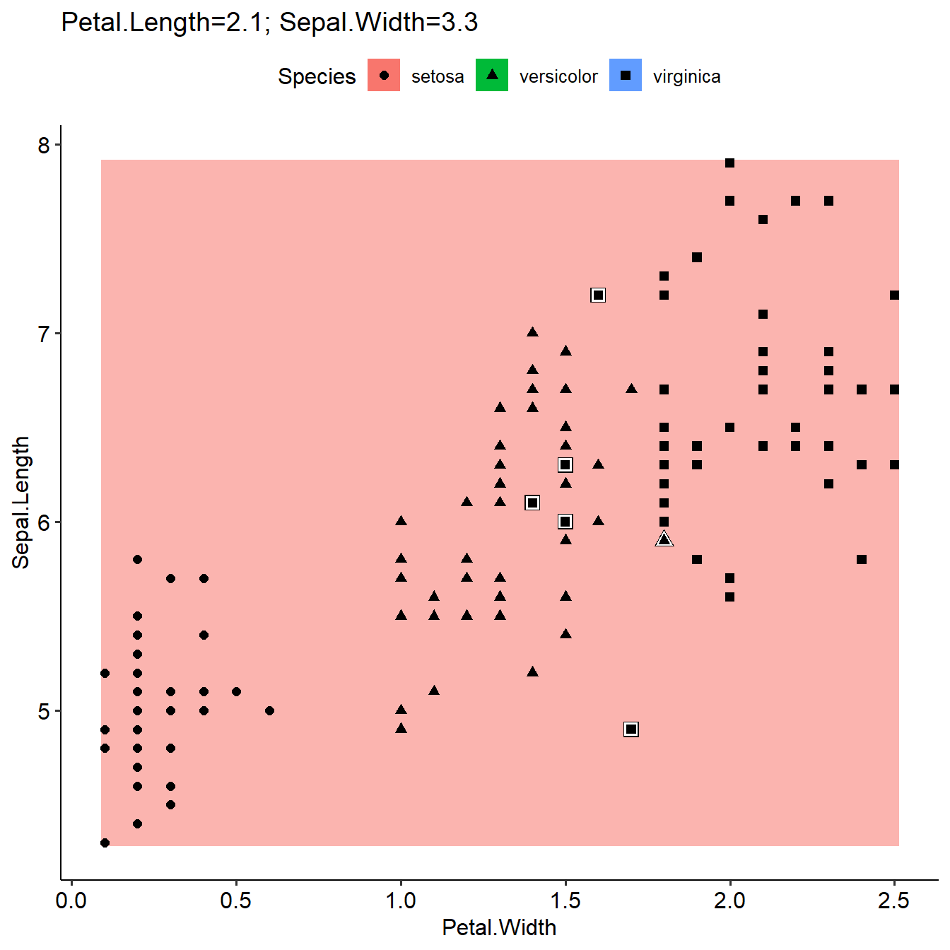
Combination of plotLearnerPrediction
It is very interesting to analyze how the distribution of prediction result among different combination of features. Here we found that although there were four features in the learner, they have different roles. “Petal.Length” was used to preidcit “setosa”; “Petal.Width” was used to predict “virginica”. “Sepal.Width” and “Sepal.Length” didn’t contribute in this model.
I like this figure (go through all combination of features and see how the preidcition results look like) and going to make this as a function too.
p1=plotLearnerPrediction(learner=learner,task=task,prob.alpha = TRUE, interestedFeatures= c("Sepal.Length","Petal.Length"))

p2=plotLearnerPrediction(learner=learner,task=task,prob.alpha = TRUE, interestedFeatures= c("Sepal.Length","Petal.Width"))

p3=plotLearnerPrediction(learner=learner,task=task,prob.alpha = TRUE, interestedFeatures= c("Sepal.Length","Sepal.Width"))

p4=plotLearnerPrediction(learner=learner,task=task,prob.alpha = TRUE, interestedFeatures= c("Petal.Width","Petal.Length"))

p5=plotLearnerPrediction(learner=learner,task=task,prob.alpha = TRUE, interestedFeatures= c("Petal.Width","Sepal.Width"))

p6=plotLearnerPrediction(learner=learner,task=task,prob.alpha = TRUE, interestedFeatures= c("Petal.Width","Sepal.Length"))

ggarrange(p1,p2,p3,p4,p5,p6,common.legend = TRUE,ncol=2,nrow=3)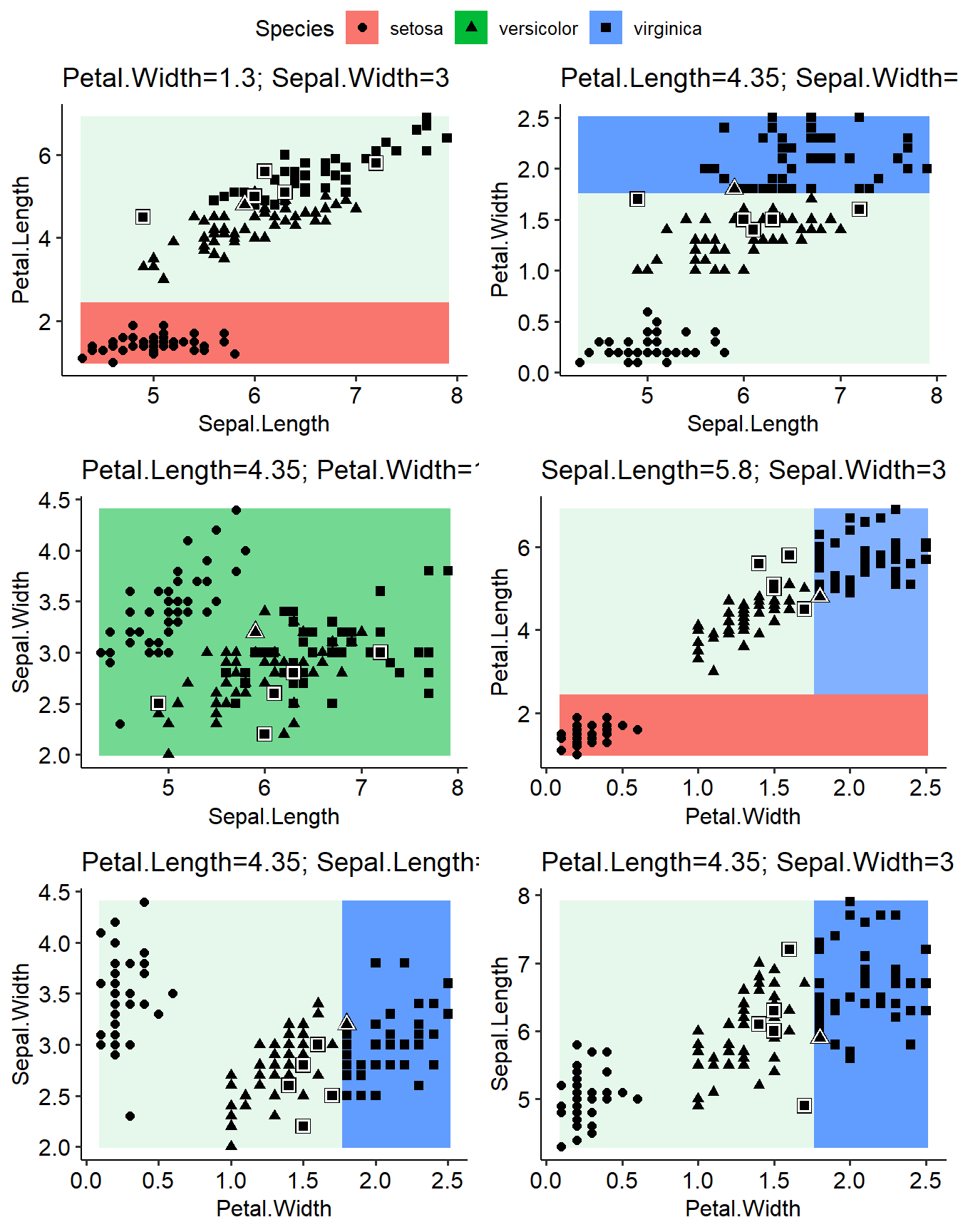
summaryFeatureInTask
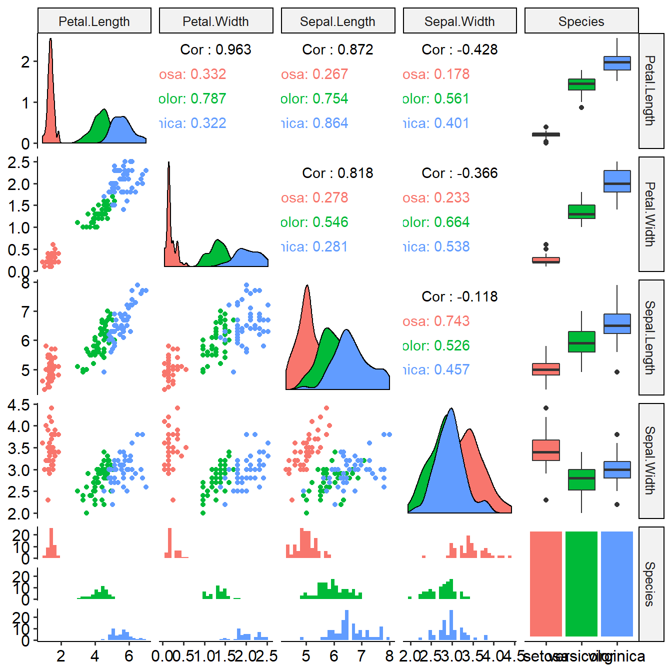
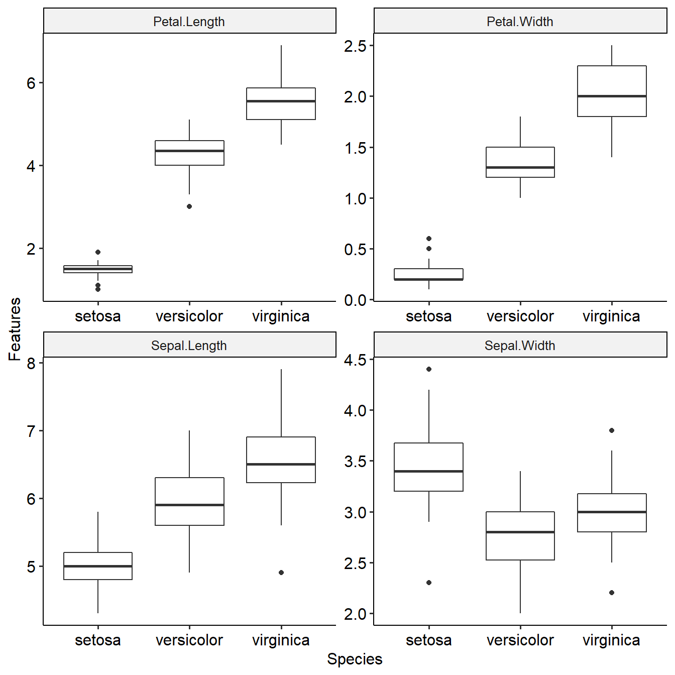
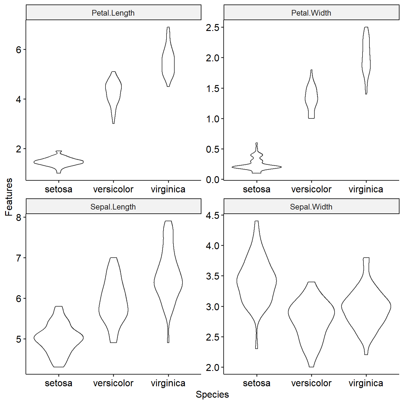
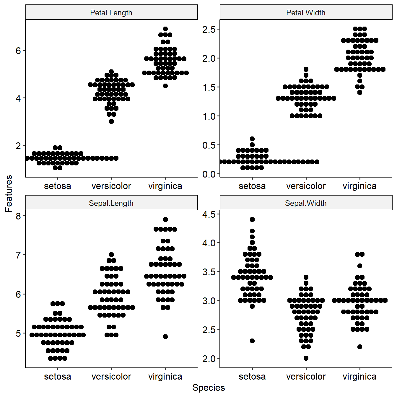
This function shows distribution of features among target groups and their differential p values. Task will be used as input.
summaryFeatureInTask(task)
#> Loading required package: lattice
#> Loading required package: survival
#> Loading required package: Formula
#>
#> Attaching package: 'Hmisc'
#> The following objects are masked from 'package:base':
#>
#>     format.pval, units
Descriptive Statistics (N=150)
| setosa (N=50) | versicolor (N=50) | virginica (N=50) | Test Statistic | |
| Petal.Length | |
|
|
F=515.64 d.f.=2,147 P<0.001 |
| Petal.Width | |
|
|
F=541.25 d.f.=2,147 P<0.001 |
| Sepal.Length | |
|
|
F=136.85 d.f.=2,147 P<0.001 |
| Sepal.Width | |
|
|
F=54.69 d.f.=2,147 P<0.001 |